A language model is model that estimating the probability p(s) of occurrence of a sentence s.
Natural Language Processing
Word sense disambiguation and uncertainty in language
- Lexical ambiguity. For example, “silver” can be a noun, an adjective, or a verb.
- Syntactic ambiguity. For example, “The man saw the girl with the telescope”. It is ambiguous whether the man saw the girl carrying a telescope or he saw her through his telescope.
- Semantic ambiguity. For example, “The car hit the dog while it was moving”. It is unclear whether the dog or the car is moving.
There are several potential phases of natural language processing. Summerized below
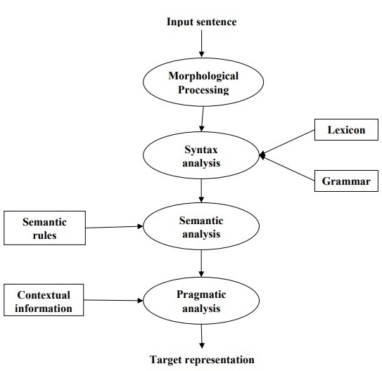
- Morphological processing refers to the cognitive mechanisms involved in recognizing and understanding the structure and meaning of words based on their constituent morphemes. Morphemes are the smallest units of meaning in a language, including prefixes, suffixes, roots, and other meaningful elements. For example, a word like “uneasy” can be broken into two sub-word tokens as “un-easy”.
- Syntax analysis, also known as parsing, is the process of analyzing the grammatical structure of sentences in natural language to determine their syntactic relationships and properties. It involves breaking down sentences into their constituent parts and representing them according to the rules of a formal grammar.
- Semantic analysis, is the process of understanding the meaning of text or speech in natural language. It involves analyzing the semantics, or meaning, of words, phrases, sentences, and larger units of discourse to extract and represent the underlying information.
- Pragmatic analysis, studies how language is used in context to convey meaning beyond the literal interpretation of words and sentences. It focuses on the social, cultural, and situational aspects of language use, as well as the intentions and beliefs of speakers and listeners.
Part-of-speech (POS) tagging is the process of assigning a specific part of speech (such as noun, verb, adjective, etc.) to each word in a given text corpus. POS tagging is essential for understanding the syntactic structure and meaning of a sentence. It helps disambiguate the meaning of words that may have multiple possible interpretations based on their context.
Text normalization
Text normalization refers to the process of transforming text into a canonical, standardized form. Some common techniques are
- Lowercasing
- Tokenization
- Removing punctuation, special characters, numbers, stop words
- Stemming
- Lemmatization
- Spelling corrections
- Handling contractions
Recurrent Neural Network
A recurrent neural network (RNN) is a class of neural networks that discover the sequential nature of the input data. Inputs could be text, speech, time series, etc.
The architecture of a simplest RNN is \(h_t=\tanh(W_{h}\cdot h_{t-1}+W_{x}\cdot x_{t}+b)\)
Types of RNN
- one-to-one: traditional neural network
- one-to-many: music generation
- many-to-one: sentiment classification
- many-to-many (equal): name entity recognition
- many-to-many (unequal): machine translation
The loss function is the sum of losses of all time steps.
Due to the number of layers in the deep neural network, the gradients as continuous matrix multiplications because of the chain rule will shrink exponentially if they start from small values (<1) and will blow up if they start from large values (>1). This is called the vanishing or exploding gradient problem.
Long Short Term Memory
Long short term memory (LSTM) is a special kind of RNN, designed to avoid long-term dependency problem. All RNN have the form of a chain of repeating modules of neural network. In standard RNNs, this repeating module has a single tanh layer, whereas LSRMs has four, interacting as below
\(\begin{cases}
f_t=\sigma(W_{fh}\cdot h_{t-1}+W_{fx}\cdot x_t+b_f) \\
i_t=\sigma(W_{ih}\cdot h_{t-1}+W_{ix}\cdot x_t+b_i) \\
o_t=\sigma(W_{oh}\cdot h_{t-1}+W_{ox}\cdot x_t+b_o) \\
\tilde C_t=\tanh(W_{Ch}\cdot h_{t-1}+W_{Cx}\cdot x_t+b_C) \\
C_t=f_t\cdot C_{t-1}+i_t\cdot \tilde C_t \\
h_t=o_t\cdot \tanh(C_t)
\end{cases}\)
Here \sigma is the sigmoid function, f_t, i_t, o_t are the forget, input, output gates, C_t is the cell state, and h_t is the hidden state.
Gated Recurrent Unit
Gated recurrent unit (GRU) is a variant of LSTM that has a simpler internal structure, and uses gating mechanisms to control and manage the flow of information between cells in the neural network. \(\begin{cases} z_t=\sigma(W_{zh}\cdot h_{t-1}+W_{zx}\cdot x_t) \\ r_t=\sigma(W_{rh}\cdot h_{t-1}+W_{rx}\cdot x_t) \\ \tilde h_t=\tanh(W_{hh}\cdot r_t h_{t-1}+W_{hx}\cdot x_t) \\ h_t=(1-z_t)\cdot h_{t-1}+z_t\cdot \tilde h_t \\ \end{cases}\)
Here r_t,\tilde h_t are the relevance, update gates.
Other variants includes
|Bidirectional (BRNN)|Deep (DRNN)|
|—|—|
| |
| |
|
Word Representations
There are two main ways of presenting words
- 1-hot representation, denoted
o_w. - word embedding, denoted
e_w.
The embedding matrix E such that e_w = Eo_w can be learnt using target/context likelihood models by defining the conditional probability as
\(p(w_o|w_i)=\frac{\exp(e_{w_o}\cdot e_{w_i})}{\sum_{w\in V}\exp(e_w\cdot e_{w_i})}\)
BOW
Bag-of-words (BOW) model treats a document as a collection of words without considering the order and the structure of the words. It is the sum of 1-hot encodings. The size of the representation huge and sparse, it also disregards the semantic understanding, and it cannot deal with out-of-vocabulary words.
TF-IDF is the product of term frequency (TF) and inverse document frequency (IDF). TF-IDF helps rank documents based on their relevance to a query. Documents containing rare or distinctive terms (with high TF-IDF scores) are considered more relevant.
n-grams are contiguous sequences of n items from a given sequence of text or speech.
Word2Vec
word2vec is a framework aimed at learning word embeddings by estimating the likelihood that a given word is surrounded by other words, popular models include
- skip-gram maximize \(\frac{1}{T}\sum_{t=1}^T\sum_{-c\leq j\leq c,j\neq0}\log p(w_{t+j}|w_t)\)
- continuous bag-of-words (CBOW) maximize \(\frac{1}{T}\sum_{t=1}^T\sum_{-c\leq j\leq c,j\neq0}\log p(w_t|w_{t+j})\)
Computing softmax probabilities for all words is computationally expensive. To address this, we could perform the computations in some other ways.
Hierarchical softmax is a way to make the calculation of the sum in the denominator of the conditional probability faster is with the help of a binary tree structure. All the leaves nodes represent words, and internal nodes measure connections between children nodes. Concretely, let n(w_o,k) to be the node on the unique path from root to w_o with w_o being its k-th generation descendant, stored with the node a weight vector v_n, we define
\(\begin{align*}
p(n\to\text{left}|w_i)&=\sigma(v_n\cdot e_i)\\
p(n\to\text{right}|w_i)&=1-p(n\to\text{left}|w_i)=\sigma(-v_n\cdot e_i)
\end{align*}\)
and
\(p(w_o|w_i)=\prod_{k}p(n(w_o,k+1)\to n(w_o,k))\)
The internal nodes embeddings are learnt during model training. The tree structure helps greatly reduce the complexity of the denominator estimation from O(V) to O(\log V).
Negative sampling transforms the objective of predicting words into a binary classification problem, the model is trained to distinguish between positive (actual context words, label y=1) and negative (randomly sampled noise, label y=0) examples. Concretely, we use probabilities
\(\begin{align*}
p(y=1|w_o,w_i)&=\sigma(e_o\cdot e_i)\\
p(y=0|w_o,w_i)&=1-\sigma(e_o\cdot e_i)=\sigma(-e_o\cdot e_i)
\end{align*}\)
Here \sigma(x)=\dfrac{1}{1+e^{-x}} is the sigmoidal function. We define the loss to be
\(\mathcal L=-\sum_{i,o}\log p(y=1|w_o,w_i)+\sum_{i,o}\sum_{w\sim P_n}\log p(y=0|w,w_i)\)
Here w\sim P_n is a negative sampled noised words, and the noise distribution P_n(w)=U(w)^{3/4}/Z is the Zipf’s law, U meaning word frequency.
Pros & Cons
- skip-gram is better suited for rare words because rare words often have unique contexts.
- skip-gram is known for capturing fine-grained semantic relationships between words. Since it learns separate embeddings for each word, which can represent subtle semantic nuances and capture relationships between words that may appear in diverse contexts.
- CBOW is faster to train. Since it aggregates context information from multiple words to predict a single target word. This approach tends to be computationally more efficient, especially for large vocabularies.
- CBOW performs better for frequent words because it average context vectors. Frequent words tend to occur in various contexts, and CBOW can effectively aggregate this information to learn robust representations for these words.
- skip-gram tends to perform better with larger datasets, while CBOW may perform better with smaller datasets.
GloVe
GloVe (global vectors) is a word embedding technique that uses a co-occurence matrix X where each X_{ij} denotes the number of times w_j occurs in the context of w_i. The co-occurrence probability is defined to be
\(P_{ij}=p(w_j|w_i)=\frac{X_{ij}}{X_i}\)
Here X_i=\sum_kX_{ik} is the number of occurrence of w_i. Define
\(F(w_i,w_j,w_k)=\frac{P_{ik}}{P_{jk}}\)
This ratio shed some light on the corelation of the probe word w_k with the words w_i and w_j. If the ratio is large, then the probe word is related to w_i but not w_j and vice versa, it equals to 1, then w_k is likely to be unrelated to both w_i,w_j. Since we would like the linearity on the word embeddings, We expect F to satisfy
\(F((e_{w_i}-e_{w_j})\cdot e_{w_k})=\frac{F(e_{w_i}\cdot e_{w_k})}{F(e_{w_j}\cdot e_{w_k})}=\frac{P_{ik}}{P_{jk}}\)
The solution would be F=\exp, so
\(F(e_{w_i}\cdot e_{w_k})=\exp(e_{w_i}\cdot e_{w_k})\)
Hence
\(e_{w_i}\cdot e_{w_k}=\log P_{ik}=\log X_{ik} - \log X_i\)
Since \log X_i is independent of k and break the symmetry between i,k, we can add a bias term b_{w_i} to e_{w_i} to absorb -\log X_i and add b_{w_k} to e_{w_k} to make it symmetric. The cost function can then be defined simply as
\(J(\theta)=\frac{1}{2}\sum_{i,j}f(X_{ij})(e_{w_i}\cdot e_{w_j}+b_{w_i}+b_{w_j}'-\log X_{ij})^2\)
Where f(c) is a weighting function should be non-decreasing and go to zero as c\to 0. For example, with some adjustable c_{\max}
\(f(c)=\begin{cases}
\left(c/c_{\max}\right)^\alpha, &\text{if $c<c_{\max}$}\\
1, &\text{otherwise}
\end{cases}\)
Given the symmetry of e_{w_i},e_{w_j}, the final word embedding is \dfrac{e_{w_i}+e_{w_j}}{2}.
Perplexity
Perplexity quantifies how surprised the model is when it sees new data. Suppose s_1,\cdots,s_N are new sentences for testing, each with m_i words, then the perplexity is defined as
\(PP=\prod_{i=1}^N\left(\frac{1}{p(s_i)}\right)^{1/m_i}=\prod_{i=1}^N\left(\prod_{k=1}^{m_i}\frac{1}{p(w_k|w_0w_1\cdots w_{k-1})}\right)^{1/m_i}\)
Machine Translation
A naive approach is to do a greedy search, meaning choosing the most likely next word each time, until the token <EOS> is selected. This doesn’t necessarily give the best outcome.
Beam search picks the top N most likely sequence each time, N is known as the beam width. This process ends when it meets some stopping criteria, for example the token <EOS> is selected.
Beam search tends to favor shorter sequences, to avoid this, length normalization uses the loss function
\(\frac{1}{T^\alpha}\sum_{t=1}^{T}\log p(w_t|w_0,w_1,\cdots,w_{t-1})\)
on the sentence s=w_0w_1\cdots w_T.
When obtaining predicted translation \hat y that is bad, we can perform error analysis using a good translation y^*
| Case | p(y^*\|x)>p(\hat y\|x) |
p(y^*\|x)\leq p(\hat y\|x) |
|---|---|---|
| Root cause | Beam search faulty | RNN faulty |
| Remedies | Increase beam width | <ul><li>Try different achitecture</li><li>Regularize</li><li>Get more data</li></ul> |
The bilingual evaluation understudy (bleu) is a metric that quantifies how good a machine translation is by computing a similarity score
\(\text{bleu score}=(\text{brebity penalty})\times\exp\left(\frac{1}{n}\sum_{k=1}^np_k\right)\)
based on n-gram precision
\(p_n=\dfrac{\text{number of matching $n$-grams}}{\text{total number of $n$-grams}}\)
and brevity penalty is a factor that penalizes the short length translation, for example, it could be
\(\text{brevity penalty}=\begin{cases}
1,&\operatorname{len}(\hat y)\geq \operatorname{len}(y^*)\\
e^{1-\operatorname{len}(y^*)/\operatorname{len}(\hat y)},&\operatorname{len}(\hat y)<\operatorname{len}(y^*)
\end{cases}\)
Seq2Seq
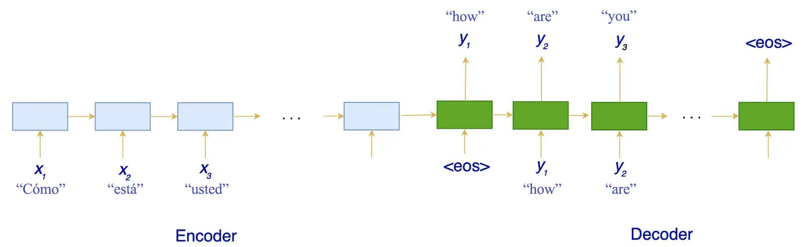
Sequence to sequence is a popular model used in tasks like machine translation, video captioning, question answering, speech recognition, etc.
It employs a encoder-decoder architecture. Both the encoder and the decoder are LSTM/GRU models. Encoder reads the input sequence and summarizes the information into context vectors. The decoder is initialized to the final state of the encoder, i.e. the context vector of the encoder’s final cell is input to the first cell of the decoder network.
Transformer
Attention
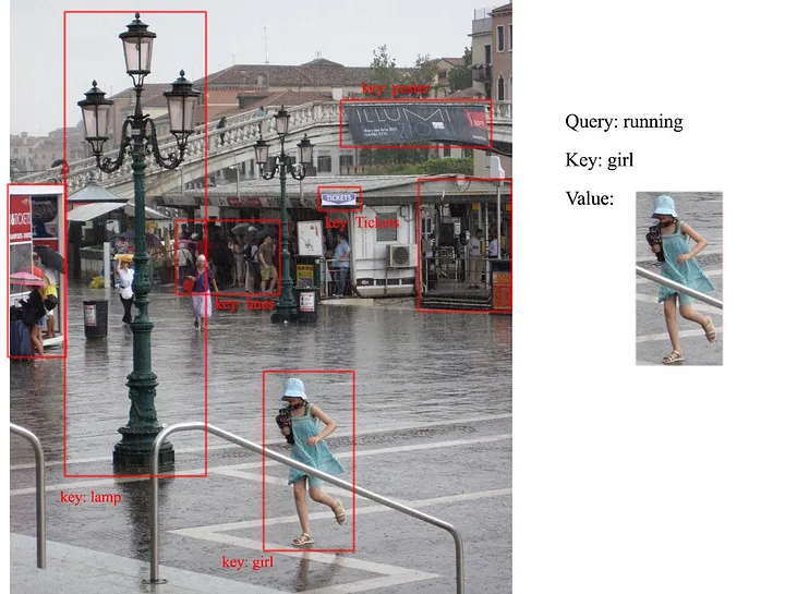
- Query
- Key
- Value
An attention function can be described as mapping a query and a set of key-value pairs to an output, where the query, keys, values, and output are all vectors. The output is computed as a weighted sum of the values, where the weight assigned to each value is computed by a compatibility function of the query with the corresponding key.
-
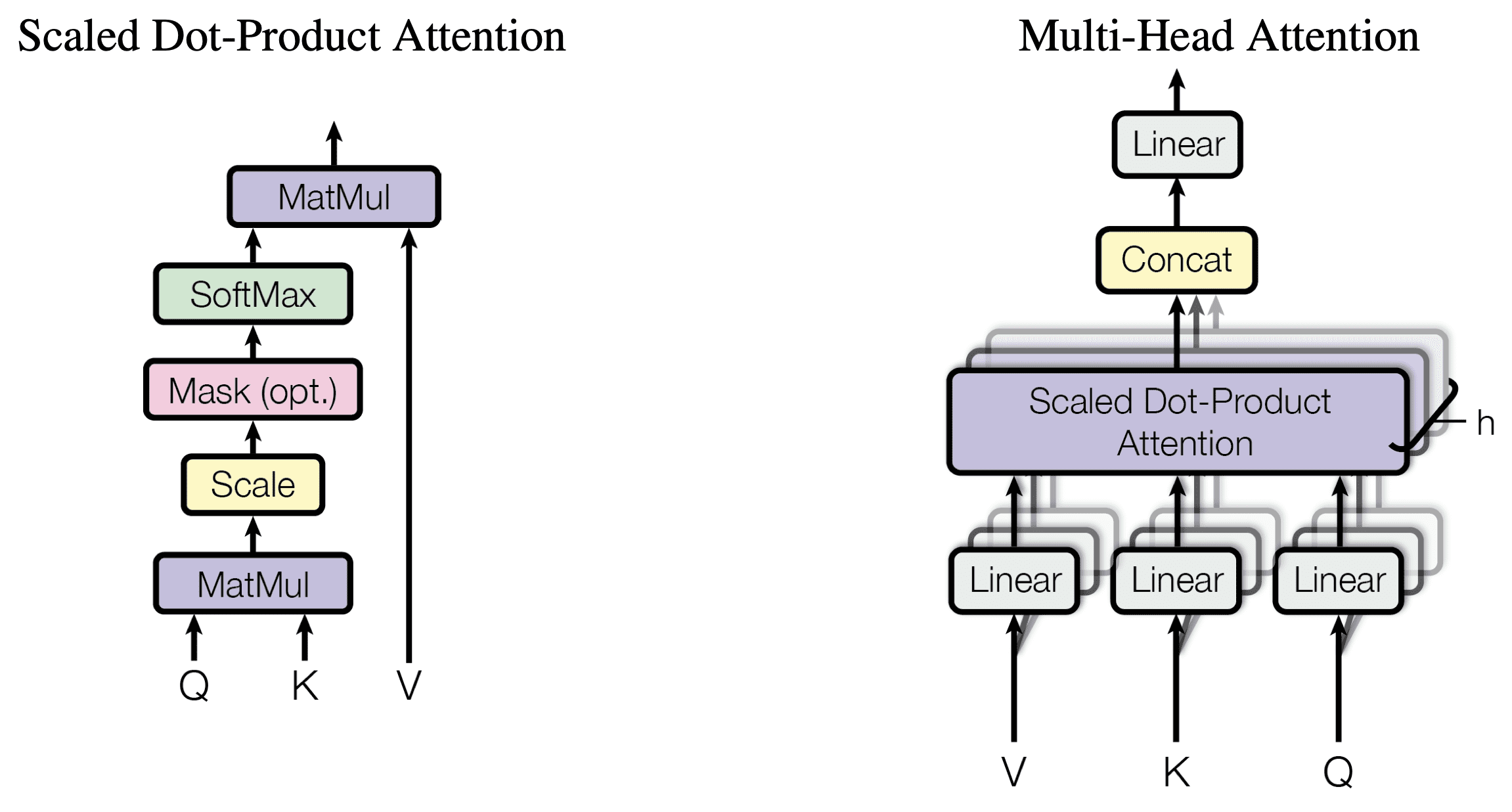
Scaled dot-product attention computes attention score as \(\text{Attention}(Q,K,V)=\operatorname{softmax}\left(\frac{QK^T}{\sqrt{d_k}}\right)V\) Here queries and keys are of dimension
d_kand values are of dimensiond_v.Another most commonly used attention function is additive \(\text{Attention}(Q,K,V)=\operatorname{softmax}(V^T\tanh(W[Q,K]+b))\) Dot-product attention is much faster and more space-efficient in practice, since it can be implemented using highly optimized matrix multiplication code
-
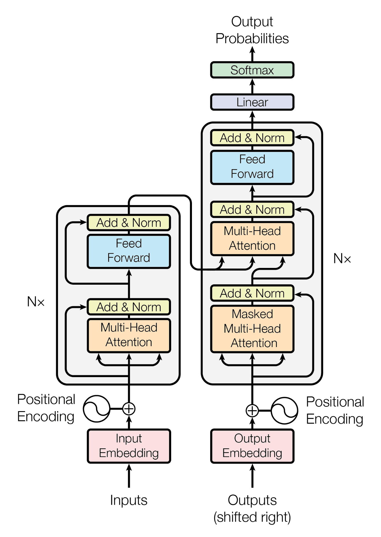
Multi-head attention instead of performing a single attention function with
d_{\text{model}}-dimensional keys, values and queries, we found it beneficial to linearly project the queries, keys and valueshtimes with different, learned linear projections tod_k,d_kandd_vdimensions, respectively. On each of these projected versions of queries, keys and values we then perform the attention function in parallel, yieldingd_v-dimensional output values. These are concatenated and once again projected, resulting in the final values.Multi-head attention allows the model to jointly attend to information from different representation subspaces at different positions. With a single attention head, averaging inhibits this. \(\begin{align*} \text{MultiHead}(Q,K,V)&=\operatorname{Concat}(\text{head}_1,\cdots,\text{head}_h)W^O\\ \text{head}_i&=\text{Attention}(QW_i^{Q},KW_i^{K},VW_i^{V}) \end{align*}\) Due to the reduced dimension of each head, the total computational cost is similar to that of single-head attention with full dimensionality.
Positional encoding
We want inject some information about the relative or absolute position of the tokens in the sequence. To this end, we add positional encodings to the input embeddings at the bottoms of the encoder and decoder stacks.
\(\begin{align*}
\text{PE}_{(\text{pos},2i)}&=\sin\left(\frac{\text{pos}}{10000^{2i/d_{\text{model}}}}\right)\\
\text{PE}_{(\text{pos},2i+1)}&=\cos\left(\frac{\text{pos}}{10000^{2i/d_{\text{model}}}}\right)
\end{align*}\)
The model easily learns to attend by relative positions, since for any fixed offset k, \text{PE}_{\text{pos}+k} can be represented as a linear function of \text{PE}_{\text{pos}}.
The architecture of the transformer model looks as follows
BERT
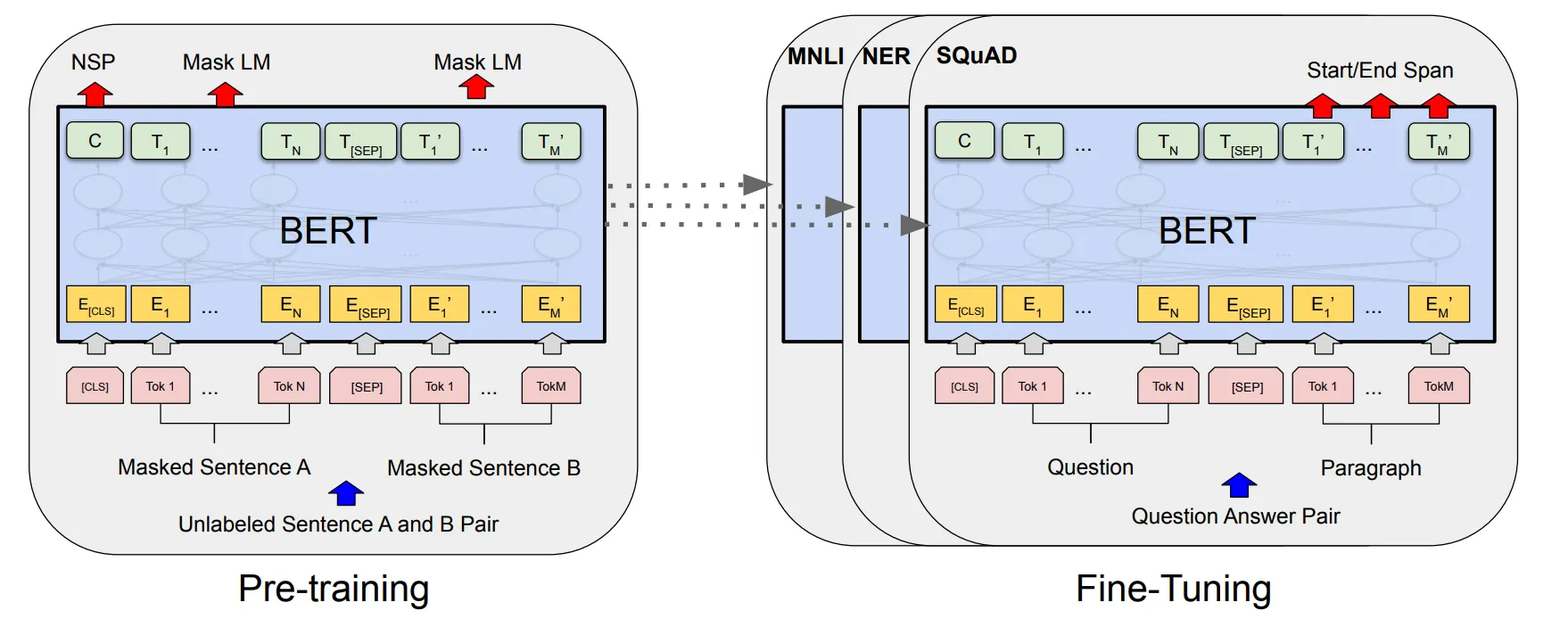
Bidirectional encoder representations from transformers (BERT) is designed to pre-train deep bidirectional representations from unlabeled text by jointly conditioning on both left and right context in all layers. As a result, the pre-trained BERT model can be fine-tuned with just one additional output layer to create models for a wide range of tasks.
Input/Output representation
Input will be in the form of a pair of sentence is represented as one token seqeunce. The first token is always [CLS], and the final hidden state vector C corresponding to this token is used as the aggregate sequence representation for classification tasks. We differentiate the pair with a [SEP] token. For a given token, its input representation is constructed by summing the corresponding token, segment, and position embeddings.

Pre-training
- Masked LM (LLM) is mask some percentage of the input tokens at random, and then predict those masked tokens. This more powerful than shallowly concatenate a left-to-right and a right-to-left model. This percentage is always taken to be 15%, for too little masking, it is too expansive in training, and for too much masking, there is not enough context.
- Next sentence prediction (NSP) tries to train the binary classification of whether sentence
Bis the next sentence of sentenceA. Here onlyCis used for this.

Domain adaptation refers to the process of adapting a model trained on data from one domain (source domain) to perform well on data from a different domain (target domain).
GAN
Generative Adversarial Networks (GAN) has two neural networks, a generator G and a discriminator D, representing the probability that x comes from the data rather than the generator. Define z to be a random noise. We want to simultaneously train D to maximize the probability of assigning the correct label to both training samples and samples from G, and train G to minimize \log(1-D(G(z))). In other words, D and G play the following minimax game with value function
\(\min_{G}\max_{D} V(D,G)=E_{x}[\log D(x)] + E_z[\log(1-D(G(z)))]\)
VAE
Variational Autoencoders (VAE)
]]>